Solar Flare Time Series Research

Introduction

I spent the summer of 2019 as a physics research intern at the Stanford University Solar Lab. I was very fortunate to have a wonderful advisor and had a great summer overall. I created machine learning models to characterize time series data for solar flare prediction. In this article, I will first provide some physics background about solar flares, then dive into my research. For a more in-depth analysis, check out the source code and my poster.

What are solar flares?

Solar flares are sudden releases of energy due to rapidly changing magnetic fields on the sun. Here is a video of a solar flare. Solar flares can release up to 10²⁵ joules of energy. To put this in perspective, the estimated world energy consumption in 2018 was about 5*10²⁰ joules; the largest solar flares release almost 20,000 times more energy than that!

Extreme ultraviolet movie of a solar flare taken by the AIA instrument.

Solar flares are a result of the sun’s constantly changing magnetic fields. The sun has many areas of strong magnetic field on its surface that rotate with the sun: these areas are called active regions. Within active regions, there may be sunspots (dark spots with a stronger magnetic field than the rest of the sun’s surface). Active regions tend to have areas of positive and negative magnetic field (like a bar magnet), so we can imagine that the magnetic field above the active region is a loop connecting the positive region to the negative region. When these loops get twisted, for example due to the movement of plasma on the sun, energy builds. The loops sometimes connect to other loops to release a burst of energy in a short period of time: this burst is a solar flare.

Scientists have been interested in properties of the sun for a long time: it is the closest star we can study! There have been two major missions for studying the sun: SOHO and SDO.

• SOHO: Solar and Heliospheric Observatory: Launched in 1995, this satellite was originally planned to be operational for only two years, however it is still running and taking data. SOHO is at the L1 point between the earth and the sun, meaning that it never changes its distance from the earth or the sun.
• SDO: Solar Dynamics Observatory: Launched in 2010, this satellite contains state-of-the-art instruments for taking beautiful pictures and magnetic data of the sun. The instrument that takes magnetic data is called HMI (Helioseismic and Magnetic Imager); the data I used for analyzing solar flares is from this instrument.

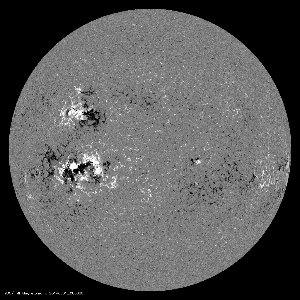Magnetogram taken by HMI: white represents positive magnetic field, black represents negative magnetic field. Note that there are distinct large patches of black and white: these are active regions.

Why should we care about solar flares?

There are both practical and scienitific reasons for studying solar flares.

First, solar flares have a direct effect on space and earth; they can produce particles in the solar wind which can alter the earth’s magnetic field and emit radiation that affects spacecraft. Solar flares are often accompanied by coronal mass ejections that can affect satellites and power grids on earth. For example, in 1989, a geomagnetic storm caused a blackout in Quebec due to variations in the Earth’s magnetic field resulting from the storm. A better understanding of the factors that cause solar flares could allow for more accurate predictions of solar weather to keep satellites and grids functional, as well as improve planning for space travel.

Second, understanding the factors behind solar flares and how the magnetically active regions of the sun change will increase our knowledge of other stars. Many stars have starspots (and therefore magnetic field patterns) similar to the sun and understanding how the active region of the sun changes would provide insight into how these other stars behave. This is important for finding stars that could have orbiting planets that support life, and for understanding differences between stars in our universe.

Why is time series important?

The problem of predicting flares is not new. My approach to the problem was different in two main ways.

1. Using time series: Much of the previous literature in the field has focused on using discrete values for flare prediction. For example, active regions with more magnetic flux tend to have a higher probability of flaring. After discussing with my advisor, I instead studied time series data. Rapid emergence of magnetic flux and free magnetic energy often indicates an increased probability of future flaring activity; if the magnetic loops get twisted faster, they are more likely to flare. It is reasonable to assume that two active regions with the same amount of magnetic flux, but different flux emergence rates have different flaring activity. I set out to model and quantify this activity.
2. Extracting physical meaning: Another goal of my project was to extract some physical meaning from the time series data. This meant choosing a model that was simple and interpretable. For this reason, I ruled out neural networks, such as LSTMs, due to to their low interpretability.

What does the data look like?

The data for this project comes from 10 years of HMI measurements aboard SDO. SDO captures and sends over a terabyte of data to earth every day. This is equivalent to amount of data the Hubble Space Telescope generates in over a month. The SDO database has amassed petabytes of data. The HMI instrument records magnetic data, which is represented in the magnetogram picture above. Since storage and analysis of data for the entire disk of the sun is expensive and cumbersome, a data product called SHARP tracks active regions and their physical properties. The SHARP database contains time series data for many different quantities calculated from the raw HMI data, including magnetic flux and active region area. I created models with the SHARP data for my project.

How do we characterize time series data for machine learning?

One of the biggest challenges for my project was featurizing the time series data. In order to do this, I first segmented the data into positive and negative classes, then used spline fitting to featurize the data segments.

1. Segmenting data: Since flaring is a binary event, I wanted to create input data for a machine learning binary classification algorithm. In order to effectively learn on time series data, all the variables are scaled (linearly) down to zero at the start of the time series data. Furthermore, I defined the positive and negative classes (note: this classification was chosen because it is similar to previous positive/negative classifications in the field) as follows:

• Positive class: A 24-hour period before a flare.
• Negative class: A 24-hour period without a flare in an active region that does flare. This last distinction is important since the problem of distinguishing between flaring and non-flaring active regions is easier than distinguishing between flaring and non-flaring regions within a flaring active region.

2. Fitting: In order to featurize the time series data, I first tried polynomial fits. I fit a polynomial using regression for each segmented 24-hour time series, then used the polynomial coefficients as features for the machine learning classifier. However, this approach is not ideal for two reasons. First, polynomial fits returned low accuracy due to Runge’s phenomenon, where small changes in the time series data could result in large changes in the polynomial coefficents. Second, the sun does not (necessarily) work according to some polynomial function over time. A better way to represent the changing variables on the sun is to use data that is divided even further. Instead of polynomial fits, I used spline fits. Spline functions are smoothed piecewise polynomials. This means that the data at the beginning of the time series will not affect the coefficients of the spline for the end of the time series. Nice!

I used the interpolated spline fit coefficients as features for a machine learning algorithm to distinguish between the positive and negative case (I specifically used B-splines due to their simplicity and interpretability). Using a stochastic gradient descent and Adaboost classifier, I was able to accurately predict whether a time series will flare according to the spline fit coefficients. Both models produced similar trends, while Adaboost had higher accuracy.

What did we learn?

For each variable recorded using the HMI instrument, I fit the variable to a model to predict flares. The features for the model (as mentioned before) are the spline fit coefficients (fit on variable vs. time data). Lag time is defined as the length of time series data used for fitting and learning. I ran trials for each variable from HMI for lag times from 2 hours to 24 hours. As lag time changed, the same positive and negative class data was used. The graph below shows the lag time versus accuracy for select variables.

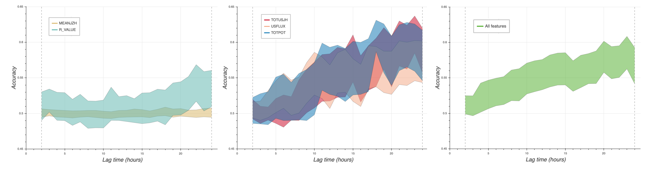Graph of accuracy lag time for select variables with error bars. Left: features where accuracy does not increase with lag time. Middle: features where accuracy increases with lag time. Right: combined feature graph.

From the graph above, it is evident that more lag time, which means more time series to learn on, improves the accuracy of the model for some features. Thus, time series is important for predicting flares; part of the signal for flares is encoded in the time series. The accuracy seems to flatten out near the 15-hour mark, however the error bars (width of the lines) are too large to make a definite conclusion. Note: although the individual accuracies of the features are low, I expect that combining the features as well as adding discrete features would yield a higher accuracy. The goal of this study was not to create the highest-accuracy model, instead it was to investigate the importance of time series data in flare prediction.

There are some variables that far outperform the others.

• The highest-performing variables are unsigned flux (USFLUX), total electric current helicity (TOTUSJH), and total free energy (TOTPOT).
  • Unsigned flux is a measure of how much magnetic field there is in an area. The formula for flux is magnetic field times area. Changing flux indicates changes in fundamental properties of the active region, so it makes sense that total flux would be a strong predictor.
  • Total electric current helicity is a measure of the rotation of the active region. It makes sense that current would be a strong predictor since changing magnetic fields cause flares, and current measures how a magnetic field is changing.
  • Total free energy is a measure of potential energy in an active region, which reflects how twisted the magnetic fields are. This is one of the best-performing features because flares are dependent upon a buildup of potential energy.
• The lowest-performing variables are mean electric current helicity (MEANJZH), and polarity inversion line flux (R_VALUE).
  • Mean electric current helicity is the average electric current helicity value across the entire active region. Since mean values are subject to more error than total values, this value is not a good predictor of flares.
  • Polarity inversion line flux is the magnetic flux near the line that divides the positive and negative regions on an active region. This feature may be a weak predictor because much of the flare signal is not located around the polarity inversion line.

What are the next steps forward?

Although the above discussion shows that time series data is important for predicting solar flares, this is by no means an exhaustive study of all the work that can be done in the future with time series analysis. In fact, this project is just a first step in time series analysis of flaring active regions. Here are a few ways that this work can be extended:

1. A polynomial or spline model does not accurately collect all the data in the time series. The sun could be better modeled by fitting the probabilities that govern how the state of different magnetic variables change. A state space model would likely produce a more robust and accurate model of the sun.
2. Further analysis can be done by changing the negative case definition. I defined the negative class as a 24-hour period without a flare. However, there could conceivably be a negative case with a flare at hour 25 (one hour after the time series). This would likely look similar to the positive case, where there is a flare at hour 24. Thus, one could explore changing the negative case to assert that there are no flares for some time after the time series data ends.
3. Lastly, the methods used in this project could be used to predict different solar events with time series data.

–

I am grateful for all the support and kindness from the Stanford solar physics group.