Introduction
I recently read Ed Thorpe’s Beat the Dealer, a book about how Thorpe, a mathematician, found a way to gain an edge in blackjack. In the book, Thorpe uses computer simulations to calculate the best blackjack strategy as well as card-counting strategies. Since I took a reinforcement learning class last quarter, I wanted to apply one of the most common algorithms, Q-learning, to to find the best strategy for blackjack.
Beat the Dealer book cover. Taken from here
Rules
In order to find the best way to play blackjack, it is essential to understand all the rules. For my simulations, I used a simplified version of blackjack where the player can only hit or stay. In a game, the player plays against the dealer. The round starts by dealing both the player and the dealer two cards. The player’s cards are dealt face up, while the dealer has one face down card and one face up card.
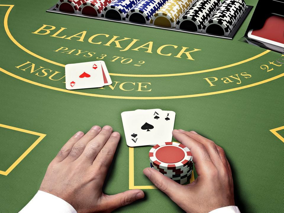
Taken from here
Winning the game
The goal of the game is for the player’s cards to sum up to as close to 21 as possible without going over 21, which is called busting. All face cards have a value of 10 and aces can take a value of either 1 or 11. The player wins if their cards are higher than the dealer’s without busting. If the dealer busts and the player doesn’t then the player wins. Else, the dealer wins.
Player actions
In the simplified version of blackjack I used for this article, after the cards are dealt, the player has a choice of two actions–they can stay or hit. If the player stays, then their turn is over. If the player hits, then they are dealt another card.
Dealer actions
The dealer’s actions are deterministic, i.e. the dealer has no agency. The dealer must hit on hands with a value of 16 or less. Furthermore, they hit on hands that have a value of 17 if one of the cards is an ace (and the ace is counted as an 11). Hands with an ace where the ace is counted as an 11 are known as “soft” hands since if the hand value goes over 21, the ace can turn into a 1. So the dealer must hit on soft 17s.
Other considerations
Another consideration that we must take into account are the number of decks. Usually there are between 1 and 8 decks at a casino. I used 6 decks for my tests.
State Space and Actions
To frame the blackjack game as a reinforcement learning problem, we have to define the set of states and the set of actions.
States
For blackjack, the only information the player has is what they can see on the table. This includes their hand and the face up dealer card (dealer hole card). Since only the values of the cards matter, we can define the state space as the value of the hand as well as the dealer hole card. However, since aces can have a value of either 1 or 11, we must include whether there is an ace in the hand that can have a value of either 1 or 11 without going over 21. As noted earlier, hands with such an ace are called soft. If the value of a certain hand is high enough, the ace is forced to be a 1 so that the player doesn’t bust. Such a hand is considered hard, not soft even though there is an ace in the hand. So our state space is the set of all possible values of hands and dealer face up cards, where the value of a hand is the sum of all the card values as well as whether the hand is soft or hard. We can therefore represent the state of a game as a tuple: (hand sum, is the hand soft, dealer hole card).
The numerical value of a hand can take on any value between 4 and 21 (18 possible values). Values of hands 12 or above can be either soft or hard, so there are 28 total possible hand values. The dealer card can take on 10 distinct values. Therefore, our state space includes 28*10=280 possible states.
Policies
As discussed before, the player has two possible actions: stay and hit. A policy is a map of states to actions. A policy decides what action to take given a state. The goal of reinforcement learning is to find the optimal policy, which is the optimal action for each state. There are therefore \(2^{280}=1.94*10^{84}\) possible policies that we could create. Clearly, iterating through all such policies would be impossible with a laptop, so we will instead find better ways to find an optimal policy.
Q-Learning
Since we can model blackjack as a Markov decision process, using reinforcement learning (RL) to learn an optimal policy is natural. I used Q-learning to find the best way to play blackjack. I will describe what Q-learning is in this section.
Q function
The \(Q\) function, or the state-action value function is central to Q-learning. \(Q\) is defined with respect to a state \(s\in\mathcal{S}\) and an action \(a\in\mathcal{A}\), where \(\mathcal{S}\) is the set of all states and \(\mathcal{A}\) is the set of all actions.
$$Q^\pi(s,a)$$
The function is parameterized by a policy \(\pi\) and represents the expected return if one starts from state \(s\), takes action \(a\) and then follows policy \(\pi\). Essentially, it represents how good an action is from a state.
Q update (learning)
A core idea that we will use for learning an optimal policy is testing out different actions, then evaluating the actions. This is represented in the following diagram:
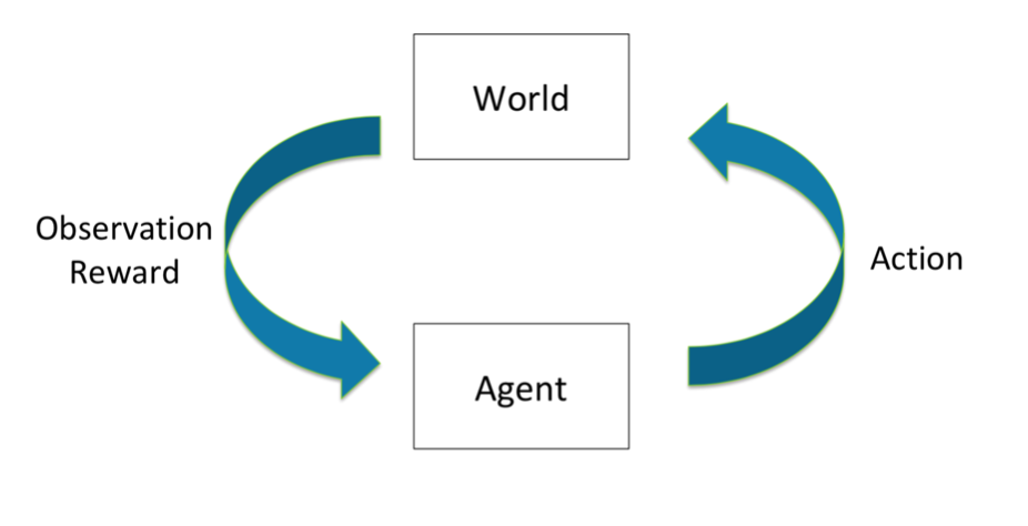 Relationship between world and agent, taken from the CS234 lecture slides (Winter 2021 lecture 4)
The \(Q\) function is updated as new data comes in. Each data point is in the form of a (state, action, reward, next state) tuple. For a timestep \(t\), this is represented as \((s_t, a_t, r_t, s_{t+1})\). Note that since we use \(Q(s_{t+1}, a)\) in the Q update, we are boostrapping. The Q update is described below.
Q update: $$Q(s_t,a_t)\leftarrow Q(s_t,a_t) + \alpha * (r_t + \gamma * \text{arg}\max_a Q(s_{t+1}, a) - Q(s_t,a_t))$$
\(\alpha\) is the learning rate, and \(\gamma\) is the discount factor. \(\alpha\) controls how fast the policy will update based on new information. \(\gamma\) controls the weighting of data in the future vs. data now. Both \(\alpha\) and \(\gamma\) are values between 0 and 1. To understand the Q update, we can break it down into simpler components.
Error term: $$r_t + \gamma * \text{arg}\max_a Q(s_{t+1}, a_t) - Q(s_t,a_t)$$
We can see that \(r_t + \gamma * \text{arg}\max_a Q(s_{t+1}, a)\) is the discounted future reward starting from state $s_t$ and taking action \(a_t\). The error term represents how far off the predicted value of the \(Q\) function is versus the stored value.
Now that we understand the \(Q\) function and the Q update, we will discuss some properties of Q-learning. These properties will be important for tuning the algorithm and acheiving good results.
Bootstrapping
Q-learning uses bootstrapping to estimate the state-value function. Bootstrapping in the context of reinforcement learning means that the model uses estimated \(Q\) function values to update the \(Q\) function. It is clear that the Q update uses bootstrapping since it uses estimated \(Q\) function values when it computes the \(Q(s_{t+1}, a)\) for all \(a\).
Model-free and off-policy
Q-learning is a model-free RL algorithm, meaning that it does not keep a “model” of the world. A model of the world is the transition probabilities and rewards between states. Q-learning, instead of keeping track of an estimated model, directly learns the \(Q\) function from the data.
Q-learning is also an off-policy RL algorithm since it estimates the value of the optimal policy while acting on a different policy. This idea is present in this term in the Q update: $$\text{arg}\max_a Q(s_{t+1}, a_t).$$ The on-policy update would be to use \(Q(s_{t+1}, a_{t+1})\). This on-policy update would estimate the value of the current policy. However, when we add the max term, we have off-policy learning.
Exploration vs. exploitation
How will we decide which actions to take in blackjack to best update our \(Q\) function? On one hand, we want to maximize the expected return from the Q function, which means we want to exploit the values we have alreadly learned. However, we also want to explore new actions in case we got unlucky in a trial, leading to an incorrect Q value. One way to balance exploration and exploitation is with an epsilon-greedy policy. For some value of \(\epsilon\) between 0 and 1, we take a random action with probability $\epsilon$ and we take the best action with probability \(1-\epsilon\). Therefore, by adjusting \(\epsilon\), we can control the amount of exploration that our agent does. We typically take \(\epsilon\) to zero after many timesteps.
Model
We will now focus on how to learn the best policy, which is the function that decides which action to take for each state. There are two steps to do model-free policy iteration: policy evaluation and policy improvement. The policy evaluation step consists of computing the Q values for a specific policy. The policy improvement step consists of updating the policy given the new Q values. Here is some pseudo-code for these two steps as used to learn a good blackjack policy:
def learn_policy():
  t = 0
  repeat NUMBER_OF_TIMESTEPS times:
    simulate 100,000 games of blackjack using the learned policy
    update Q values based on the (state, action, reward, next state) tuples from the simulations
    update the policy to be epsilon greedy with respect to the learned Q values
    t += 1
Simulating the games of blackjack and updating the Q values constitutes the policy evaluation step. The policy improvement step is simply creating the new policy with respect to the Q values.
Tuning the Model
Alpha
Recall that \(\alpha\) is the learning rate for the model. It controls how fast the Q values will be updated. To ensure that Q-learning converges to the optimal Q values, we must visit all state-action pairs infinitely often, and the step sizes $\alpha_t$ must satisfy the Robbins-Munro sequence. To satisfy the first condition, we can uniformly pick states and actions to make sure that we visit all state-action pairs infinitely often. For the second condition, we choose \(\alpha_t=1/t\). This satisfies the Robbins-Munro sequence, which is the following two inequalities: $$\sum_{t=1}^\infty\alpha_t=\infty$$ and $$\sum_{t=1}^\infty\alpha_t^2<\infty.$$
Epsilon
\(\epsilon\) is the amount of exploration we conduct with the \(\epsilon\)-greedy policy. To ensure that Q-learning converges to the optimal policy, we must visit all state-action pairs infinitely often and ensure that the $\epsilon$-greedy policy converges to a greedy policy. A common strategy to satisfy these conditions (known as GLIE) is setting \(\epsilon_t=1/t\).
Gamma
\(\gamma\) is the discount rate. I set \(\gamma\)=1 since it performed the best in trials.
Results
Now, we will see how well our Q-learning function does compared to the optimal blackjack strategy! I took the optimal strategy from this website. The optimal strategy has a win rate of 0.428 and a loss rate of 0.478.
Baselines
I used two suboptimal baseline strategies to compare against our learned policies: random strategy and stand only strategy. The random strategy has a win rate of 0.282 and a loss rate of 0.676. The stand only strategy has a win rate of 0.382 and a loss rate of 0.566.
Win rate
We will see how the Q-learning strategy compares with the baselines as well as the optimal strategy after many time steps. Here is a plot of the win rate of the Q-learning strategy versus number of time steps. Each time steps is 100,000 games of blackjack.
 Win rate versus number of time steps
We can see that the Q-learning strategy reaches the optimal win rate in around 50 time steps. Furthermore, as time goes on, the win rate seems to stabilize, indicating it is converging on the optimal strategy.
Policy
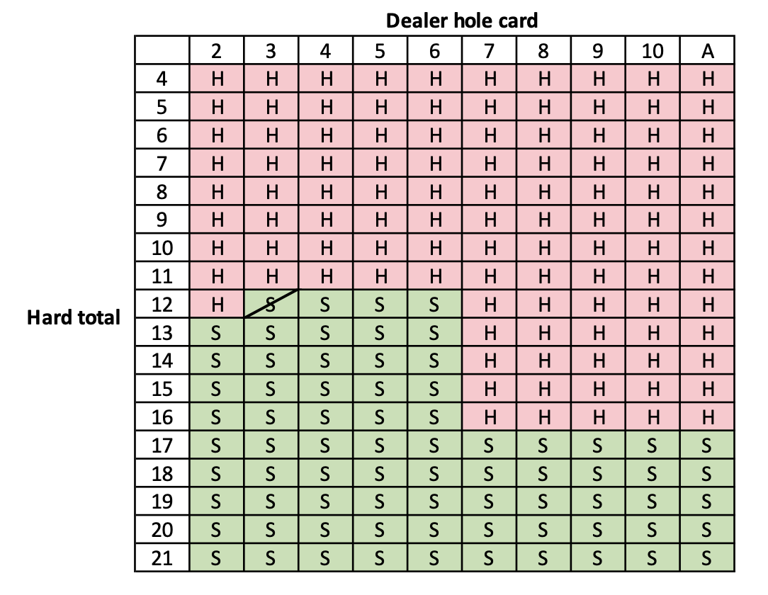
Here is the optimal policy for the game. S=stand and H=hit.
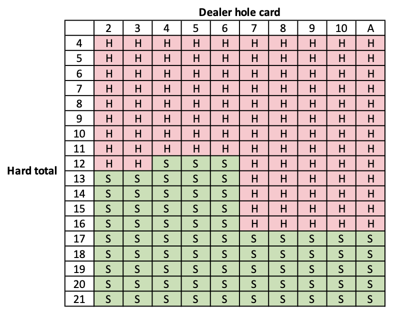 Hard total optimal policy
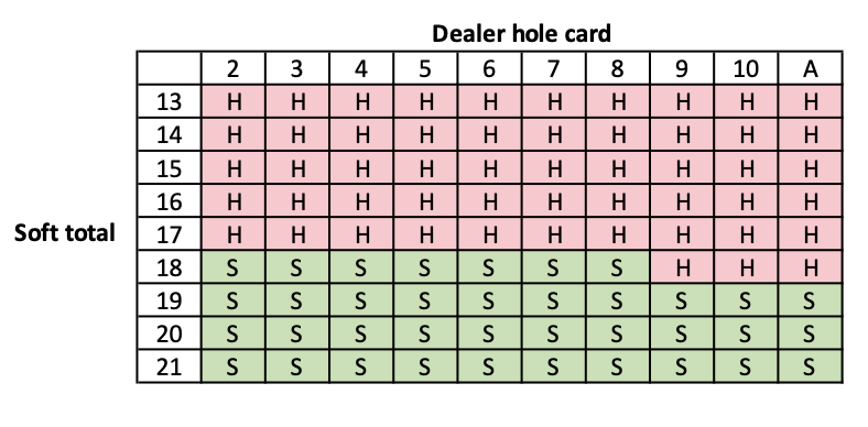 Soft total optimal policy
Here is the learned policy for the game after 250 iterations. Places where the learned policy deviates from the optimal policy are crossed out.
 Hard total learned policy
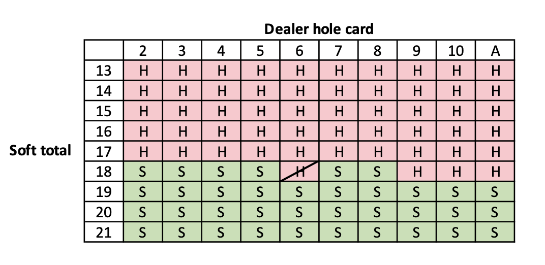 Soft total learned policy
As we can see, our learned policy is very close to the optimal policy: we have two total errors. We can see from the win rate vs. time steps graph that this small variation in policy does not affect the win rate much. I believe that with more time steps, it is possible to achieve the optimal policy.
Conclusion
I hope that this article gave some insight into Q-learning and showed an application for the algorithm. Here is the code I used for my simulation: https://github.com/lucaspauker/blackjack_reinforcement_learning. Feel free to play with it and see if there is a way to improve the algorithm.